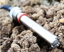
Dissolved Oxygen sensor
Products
Dissolved oxygen analysis measures the amount of gaseous oxygen (O2) dissolved in an aqueous solution. Oxygen gets into water by diffusion from the surrounding air, by aeration (rapid movement), and as a waste product of photosynthesis. When performing the dissolved oxygen test, only grab samples should be used, and the analysis should be performed immediately. Therefore, this is a field test that should be performed on site.
All animals need oxygen to survive. Dissolved oxygen is what makes aquatic life possible. Changes in oxygen concentration may affect species dependent on oxygen-rich water, like many macroinvertebrate species. Without sufficient oxygen they may die, disrupting the food chain. Oxygen concentration can also affect other chemicals in the water. For example, cadmium stays in a solid form in the presence of oxygen and sinks to the bottom of the water. However, if the water goes anoxic (without oxygen) cadmium may dissolve into the water. This is a problem because cadmium (as with other hard metals) is poisonous to animals.
Total dissolved gas concentrations in water should not exceed 110%. Concentrations above this level can be harmful to aquatic life. Fish in waters containing excessive dissolved gases may suffer from “gas bubble disease”; however, this is a very rare occurrence. The bubbles or emboli block the flow of blood through blood vessels causing death. External bubbles (emphysema) can also occur and be seen on fins, on skin and on other tissue. Aquatic invertebrates are also affected by gas bubble disease but at levels higher than those lethal to fish.
Adequate dissolved oxygen is necessary for good water quality. Oxygen is a necessary element to all forms of life. Natural stream purification processes require adequate oxygen levels in order to provide for aerobic life forms. As dissolved oxygen levels in water drop below 5.0 mg/l, aquatic life is put under stress. The lower the concentration, the greater the stress. Oxygen levels that remain below 1-2 mg/L for a few hours can result in large fish kills.
Dissolved oxygen sensors, both electrochemical and optical, do not measure the concentration of dissolved oxygen in mg/L or ppm (parts per million which is equivalent to mg/L). Instead, the sensors measure the pressure of oxygen that is dissolved in the sample. To simplify the readings displayed by an instrument, the pressure of the dissolved oxygen is expressed as DO% Saturation.
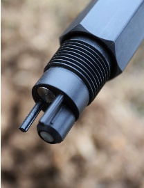
Electrochemical sensors, both polarographic and galvanic, consist of an anode and a cathode that are confined in electrolyte solution by an oxygen permeable membrane. Oxygen molecules that are dissolved in the sample diffuse through the membrane to the sensor at a rate proportional to the pressure difference across it. The oxygen molecules are then reduced at the cathode producing an electrical signal that travels from the cathode to the anode and then to the instrument.
Since oxygen is rapidly reduced or consumed at the cathode, it can be assumed that the oxygen pressure under the membrane is zero. Therefore, the amount of oxygen diffusing through the membrane is proportional to the partial pressure of oxygen outside the membrane.
A major difference between polarographic and galvanic sensors is that the galvanic sensor does not require a polarizing voltage to be applied in order to reduce the oxygen that has passed through the membrane. Rather, the electrode materials for the galvanic sensor have been chosen so that their electrode potentials are dissimilar enough to reduce oxygen without an applied voltage.
Given that the galvanic sensor does not require an external voltage for polarization, it therefore does not require the “warm-up” polarization time that the polarographic sensor requires. Since a galvanic sensor doesn’t require a “warm-up” time, the instrument is ready to measure when it is powered on and, therefore, users are not required to wait to calibrate or to take readings when using a galvanic sensor. Conversely, when an instrument with a polarographic sensor is turned on, the polarizing potential is applied to the sensor and a substantial “warm-up” period is required before the sensor is stable enough for calibration and measurements. Thus, there is an advantage of galvanic sensors over polarographic sensors in terms of convenience of use.
Winkler Method
The Winkler method involves filling a sample bottle completely with water (no air is left to bias the test). The dissolved oxygen is then “fixed” using a series of reagents that form an acid compound that is titrated. Titration involves the drop-by-drop addition of a reagent that neutralizes the acid compound and causes a change in the color of the solution. The point at which the color changes is the “endpoint” and is equivalent to the amount of oxygen dissolved in the sample. The sample is usually fixed and titrated in the field at the sample site. It is possible, however, to prepare the sample in the field and deliver it to a lab for titration.
Dissolved oxygen field kits using the Winkler method are relatively inexpensive, especially compared to a meter and probe. You can also buy the reagents in larger quantities, in bottles, and measure them out with a volumetric scoop. The advantage of the pillows is that they have a longer shelf life and are much less prone to contamination or spillage. The advantage of buying larger quantities in bottles is that the cost per test is considerably less.
The major factor in the expense of the kits is the method of titration they use eyedropper, syringe-type titrator, or digital titrator. Eyedropper and syringe-type titration is less precise than digital titration because a larger drop of titrant is allowed to pass through the dropper opening and, on a micro-scale, the drop size (and thus the volume of titrant) can vary from drop to drop. A digital titrator or a buret (which is a long glass tube with a tapered tip like a pipet) permits much more precision and uniformity in the amount of titrant that is allowed to pass.
If your program requires a high degree of accuracy and precision in DO results, use a digital titrator. A kit that uses an eye dropper-type or syringe- type titrator is suitable for most other purposes. The lower cost of this type of DO field kit might be attractive if you are relying on several teams of volunteers to sample multiple sites at the same time.
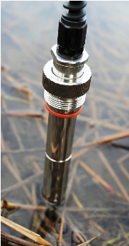
Meter and Probe
A dissolved oxygen meter is an electronic device that converts signals from a probe that is placed in the water into units of DO in milligrams per liter. Most meters and probes also measure temperature. The probe is filled with a salt solution and has a selectively permeable membrane that allows DO to pass from the stream water into the salt solution. The DO that has diffused into the salt solution changes the electric potential of the salt solution and this change is sent by electric cable to the meter, which converts the signal to milligrams per liter on a scale that the volunteer can read.
TABLE I.
Solubility of oxygen in mg/L as a function of temperature (mount air barometric pressure = 760 mm Hg, salinity = 0.0 ppt) (Source: EIFAC, 1986)| Temp (°C) | 0.0 | 0.1 | 0.2 | 0.3 | 0.4 | 0.5 | 0.6 | 0.7 | 0.8 | 0.9 |
|---|---|---|---|---|---|---|---|---|---|---|
| 0 | 14.602 | 14.561 | 14.520 | 14.479 | 14.438 | 14.398 | 14.358 | 14.318 | 14.278 | 14.238 |
| 1. | 14.198 | 14.159 | 14.120 | 14.081 | 14.042 | 14.004 | 13.969 | 13.927 | 13.889 | 13.851 |
| 2. | 13.813 | 13.776 | 13.738 | 13.701 | 13.664 | 13.627 | 13.591 | 13.554 | 13.518 | 13.482 |
| 3. | 13.445 | 13.410 | 13.374 | 13.338 | 13.303 | 13.268 | 13.233 | 13.198 | 13.163 | 13.128 |
| 4. | 13.094 | 13.060 | 13.025 | 12.991 | 12.957 | 12.924 | 12.890 | 12.857 | 12.823 | 12.790 |
| 5. | 12.757 | 12.725 | 12.692 | 12.659 | 12.627 | 12.595 | 12.563 | 12.531 | 12.499 | 12.467 |
| 6. | 12.436 | 12.404 | 12.373 | 12.342 | 12.311 | 12.280 | 12.249 | 12.218 | 12.188 | 12.158 |
| 7. | 12.127 | 12.097 | 12.067 | 12.037 | 12.008 | 11.978 | 11.949 | 11.919 | 11.980 | 11.861 |
| 8. | 11.832 | 11.803 | 11.774 | 11.746 | 11.717 | 11.689 | 11.661 | 11.632 | 11.604 | 11.577 |
| 9. | 11.549 | 11.521 | 11.493 | 11.466 | 11.439 | 11.412 | 11.384 | 11.357 | 11.331 | 11.304 |
| 10. | 11.277 | 11.251 | 11.224 | 11.198 | 11.172 | 11.145 | 11.119 | 11.093 | 11.068 | 11.042 |
| 11. | 11.016 | 10.991 | 10.995 | 10.940 | 10.915 | 10.890 | 10.865 | 10.864 | 10.815 | 10.791 |
| 12. | 10.766 | 10.741 | 10.717 | 10.693 | 10.669 | 10.645 | 10.620 | 10.597 | 10.573 | 10.549 |
| 13. | 10.525 | 10.502 | 10.478 | 10.455 | 10.432 | 10.409 | 10.386 | 10.363 | 10.340 | 10.317 |
| 14. | 10.294 | 10.271 | 10.249 | 10.226 | 10.204 | 10.182 | 10.160 | 10.137 | 10.115 | 10.094 |
| 15. | 10.072 | 10.050 | 10.028 | 10.007 | 9.985 | 9.964 | 9.942 | 9.921 | 9.900 | 9.879 |
| 16. | 9.858 | 9.837 | 9.816 | 9.795 | 9.774 | 9.753 | 9.733 | 9.712 | 9.692 | 9.672 |
| 17. | 9.651 | 9.631 | 9.611 | 9.591 | 9.571 | 9.551 | 9.531 | 9.512 | 9.492 | 9.472 |
| 18. | 9.453 | 9.433 | 9.414 | 9.395 | 9.375 | 9.356 | 9.337 | 9.318 | 9.299 | 9.280 |
| 19. | 9.261 | 9.242 | 9.224 | 9.205 | 9.187 | 9.168 | 9.150 | 9.131 | 9.113 | 9.095 |
| 20. | 9.077 | 9.058 | 9.040 | 9.022 | 9.004 | 8.987 | 8.969 | 8.951 | 8.933 | 8.916 |
| 21. | 8.989 | 8.881 | 8.863 | 8.846 | 8.829 | 8.812 | 8.794 | 8.777 | 8.760 | 8.743 |
| 22. | 8.726 | 8.709 | 8.693 | 8.676 | 8.659 | 8.642 | 8.626 | 8.609 | 8.583 | 8.576 |
| 23. | 8.560 | 8.544 | 8.528 | 8.511 | 8.495 | 8.479 | 8.463 | 8.447 | 8.431 | 8.415 |
| 24. | 8.400 | 8.384 | 8.368 | 8.352 | 8.337 | 8.321 | 8.306 | 8.290 | 8.275 | 8.260 |
| 25. | 8.244 | 8.29 | 9.214 | 8.199 | 8.184 | 8.168 | 8.153 | 8.139 | 8.124 | 8.109 |
| 26. | 8.094 | 8.079 | 9.065 | 8.050 | 8.035 | 8.021 | 8.006 | 7.992 | 7.977 | 7.963 |
| 27. | 7.949 | 7.934 | 7.920 | 7.906 | 7.892 | 7.878 | 7.864 | 7.850 | 7.836 | 7.822 |
| 28. | 7.808 | 7.794 | 7.780 | 7.766 | 7.753 | 7.739 | 7.725 | 7.712 | 7.698 | 7.685 |
| 29. | 7.671 | 7.658 | 7.645 | 7.631 | 7.618 | 7.605 | 7.592 | 7.578 | 7.565 | 7.552 |
| 30. | 7.539 | 7.526 | 7.513 | 7.500 | 7.487 | 7.475 | 7.462 | 7.449 | 7.436 | 7.424 |
| 31. | 7.411 | 7.398 | 7.386 | 7.373 | 7.361 | 7.348 | 7.336 | 7.324 | 7.311 | 7.299 |
| 32. | 7.287 | 7.274 | 7.262 | 7.250 | 7.238 | 7.226 | 7.214 | 7.202 | 7.190 | 7.178 |
| 33. | 7.166 | 7.154 | 7.142 | 7.130 | 7.119 | 7.107 | 7.095 | 7.083 | 7.072 | 7.060 |
| 34. | 7.049 | 7.037 | 7.026 | 7.014 | 7.003 | 6.991 | 6.980 | 6.969 | 6.957 | 6.946 |
| 35. | 6.935 | 6.924 | 6.912 | 6.901 | 6.890 | 6.879 | 6.868 | 6.857 | 6.846 | 6.835 |
| 36. | 6.824 | 6.813 | 6.802 | 6.791 | 6.781 | 6.770 | 6.759 | 6.748 | 6.738 | 6.727 |
| 37. | 6.716 | 6.706 | 6.695 | 6.685 | 6.674 | 6.664 | 6.653 | 6.643 | 6.632 | 6.622 |
| 38. | 6.612 | 6.601 | 6.591 | 6.581 | 6.570 | 6.560 | 6.550 | 6.540 | 6.530 | 6.520 |
| 39. | 6.509 | 6.499 | 6.489 | 6.479 | 6.469 | 6.460 | 6.450 | 6.440 | 6.430 | 6.420 |
| 40. | 6.410 | 6.400 | 6.391 | 6.381 | 6.371 | 6.361 | 6.352 | 6.342 | 6.333 | 6.323 |
TABLE II.
Solubility of oxygen, nitrogen, and argon (mg/L) as a function of depth (moist air, T = 20°C, salinity = 0.0 ppt, p = 760 mm Hg) (source: EIFAC, 1986)| Depth m | N2+Ar | O2 | Total |
|---|---|---|---|
| 0.00 | 15.43 | 9.08 | 24.51 |
| 0.10 | 15.58 | 9.17 | 24.75 |
| 0.20 | 15.74 | 9.26 | 24.99 |
| 0.30 | 15.89 | 9.35 | 25.24 |
| 0.40 | 16.04 | 9.44 | 24.48 |
| 0.50 | 16.19 | 9.53 | 25.72 |
| 0.60 | 16.35 | 9.62 | 25.96 |
| 0.70 | 16.50 | 9.71 | 26.21 |
| 0.80 | 16.65 | 9.80 | 26.45 |
| 0.90 | 16.80 | 9.89 | 26.69 |
| 1.00 | 16.96 | 9.98 | 26.93 |
| 1.10 | 17.11 | 10.07 | 27.18 |
| 1.20 | 17.27 | 10.16 | 27.42 |
| 1.30 | 17.41 | 10.25 | 27.66 |
| 1.40 | 17.57 | 10.34 | 27.90 |
| 1.50 | 17.72 | 10.43 | 28.15 |
| 1.60 | 17.87 | 10.52 | 28.39 |
| 1.70 | 18.02 | 10.61 | 28.63 |
| 1.80 | 18.18 | 10.69 | 28.87 |
| 1.90 | 18.33 | 10.78 | 29.11 |
| 2.00 | 18.48 | 10.87 | 29.36 |
| 2.10 | 18.64 | 10.96 | 29.60 |
| 2.20 | 18.79 | 11.05 | 29.84 |
| 2.30 | 18.94 | 11.14 | 30.08 |
| 2.40 | 19.09 | 11.23 | 30.33 |
| 2.50 | 19.25 | 11.32 | 30.57 |
| 2.60 | 19.40 | 11.41 | 30.81 |
| 2.70 | 19.55 | 11.50 | 31.05 |
| 2.80 | 19.70 | 11.59 | 31.30 |
| 2.90 | 19.86 | 11.68 | 31.54 |
| 3.00 | 20.01 | 11.77 | 31.78 |
| 3.10 | 20.16 | 11.86 | 32.02 |
| 3.20 | 20.31 | 11.95 | 32.27 |
| 3.30 | 20.47 | 12.04 | 32.51 |
| 3.40 | 20.62 | 12.13 | 32.75 |
| 3.50 | 20.77 | 12.22 | 32.99 |
| 3.60 | 20.92 | 12.31 | 33.24 |
| 3.70 | 21.08 | 12.40 | 33.48 |
| 3.80 | 21.23 | 12.49 | 33.72 |
| 3.90 | 21.38 | 12.58 | 33.96 |
| 4.00 | 21.53 | 12.67 | 34.21 |